Practice Set: Tidyverse
Tidyverse
Without data, there would be no science. Without clean data, there would be no analysis! Just because researchers have data does not mean they can simply throw it into a regression and be done with it.
In reality, researchers spend much more time cleaning and preparing their data than actually analyzing it: up to 80% of the time spent on data analysis tasks dealt with simply cleaning data (Dasu & Johnson, 2003)!
Evidently, data cleaning is vital to research, but it is not as difficult as it may seem! Fortunately, the collection of R packages in Tidyverse make data cleaning incredibly less arduous and painstaking; therefore, learning how to work with Tidyverse will make your life all the more simple.
dplyr
The first (and arguably most important) of Tidyverse’s core packages is dplyr. Of this package, we will focus on the five functions arguably most vital for data cleaning:
- filter()
- select()
- mutate()
- summarise()
- group_by()
We will begin with using dplyr on the steam_hw dataset. The data comes from researcher Hao Lin at Tianjin University of Technology (Lin, 2024). Broadly, their research revolves around relationships between Big Five personality traits and online gaming behavior, primarily Steam platform activity.
Loading in the data
When you load in the dataset, the first column (usually labeled …1
if using read_csv()) contains values indexing the row number, which is
redundant with the row names of the data frame that already show this.
I like to remove this column to reduce clutter, and we can do that by
using the select() function.
Hint
Remember from the lecture that select() can not only be used to choose
which columns you want to keep, but also ones you want to get rid of:
You try!
What is the code for viewing the age column?
We can see here that there are 3 participants not from China. I want
to remove them from the data set, and I can do that using filter().
steam_china_1 <- steam_hw |>
  filter(country == "china")
Filtering the data
Since this data was collected from a Chinese institution, I may be interested in looking at the gaming behavior of only Chinese participants.
To make sure I am only making inferences on Chinese participants, we would need to filter() participants who are only from China.
We can quickly view the contents of only the country column by
using the select() function.
steam_hw |>
  select(country) |>
  print()
## # A tibble: 171 × 1
## country
## <chr>
## 1 china
## 2 china
## 3 china
## 4 china
## 5 china
## 6 china
## 7 china
## 8 china
## 9 china
## 10 china
## # ℹ 161 more rowsYou try!
What if I wanted to have a data frame with only people from Guatemala? Store this as an object called steam_guatemala.
If we look at this new data frame, our number of participants (i.e., rows) dropped from 171 to 149. This is much more than just 3 participants that we are removing.
What happened? Is there something wrong with the filter() function?
There are a couple ways we can tackle this, and they involve using logical operators.
We could, instead, filter out the other countries that are not China:
steam_china_2 <- steam_hw |>
  filter(!(country == "Afghanistan" | country == "Australia" | country == "Guatemala"))
There are a couple of things to notice with the above code chunk.
I used ! with filter: the ! means “not”, so I am keeping the observations that are not following the subsequent filter specifications.
Because there are 3 different countries in the country column that I am not interested in, I need to list these 3 in the
filter()function. For this to work, I used “|” which means “or”. So I am only keeping participants who did not respond with Afghanistan or Australia or Guatemala.
This won’t be the most efficient way if there are more than 3 countries
you would have to specify in the filter() command.
You try!
What is another way to filter for participants from China
that takes this spelling difference into consideration? Call the output steam_china.
Hint: Remember the logical operators.
Regardless, we now have a data frame with 168 observations: 3 less than the 171 we initially worked with, showing that we have now filtered the correct number of participants.
You try!
If I wanted to filter for participants that are both from China and female, how could I do this? Call the result
steam_china_femaleWhat about males who are 18-25 years old? Call the result
steam_young_male
Hint: Remember the logical operators.
Personality variables
One of the standard ways of assessing the Big Five personality traits is by using the BFI-2 inventory (John & Soto, 2017), which contains 12 items per personality trait (12 items times 5 traits = 60 total items), with each item measured on a scale from 1 to 5 (1 = strongly disagree and 5 = strongly agree).
In case you are not familiar, the Big Five contains these traits:
- Extraversion
- Agreeableness
- Conscientiousness
- Neuroticism
- Openness
Looking back at our data frame, we see that participants’ scores on each item corresponds to the columns labeled with a letter, representing the trait, a number, and another letter. Just looking at individual items won’t tell us, for example, how extraverted a participant is; instead, we need some variable that gives us a combined score of the relevant items to get a personality trait score.
A simple metric is to take the sum of numeric response from each item, so participants will have a combined score of how extraverted they are (e.g., 52 out of 60 possible).
So, let us make 5 new variables that will give us the sum of participant’s trait scores along each of the 5 personality traits.
To do so, we need to sum across the items that correspond to each trait, separately (e.g., all Extraversion items summed together, all Agreeableness items, etc.). To do this, we can use across() which will apply a function over multiple columns, and combine that with the selecting function starts_with(), which we can use to specify which columns we want to sum across for each of the new variables we will create.
These functions are all nested within the mutate() command, which will add these new columns to the data frame:
china_sum_1 <- steam_china |>
  mutate(
    Extra_sum = sum(across(starts_with("E_")), na.rm = TRUE),
    Agre_sum = sum(across(starts_with("A_")), na.rm = TRUE),
    Cons_sum = sum(across(starts_with("C_")), na.rm = TRUE),
    Neuro_sum = sum(across(starts_with("N_")), na.rm = TRUE),
    Open_sum = sum(across(starts_with("O_")), na.rm = TRUE)
  )

kable(china_sum_1[c(1:10), c(1, 73:77)])| id | Extra_sum | Agre_sum | Cons_sum | Neuro_sum | Open_sum |
|---|---|---|---|---|---|
| 1 | 5789 | 7200 | 6614 | 5709 | 7127 |
| 2 | 5789 | 7200 | 6614 | 5709 | 7127 |
| 3 | 5789 | 7200 | 6614 | 5709 | 7127 |
| 4 | 5789 | 7200 | 6614 | 5709 | 7127 |
| 5 | 5789 | 7200 | 6614 | 5709 | 7127 |
| 6 | 5789 | 7200 | 6614 | 5709 | 7127 |
| 7 | 5789 | 7200 | 6614 | 5709 | 7127 |
| 8 | 5789 | 7200 | 6614 | 5709 | 7127 |
| 9 | 5789 | 7200 | 6614 | 5709 | 7127 |
| 10 | 5789 | 7200 | 6614 | 5709 | 7127 |
In this new data frame, we successfully summed across the proper items, but the sum we get is MUCH larger than we would expect, and it is the same for every participant. We want to get the sum for each participant, not the total across all participants.
To do this, we need to make use of the group_by() function:
china_sum_2 <- steam_china |>
  group_by(id) |>
  mutate(
    Extra_sum = sum(across(starts_with("E_")), na.rm = TRUE),
    Agre_sum = sum(across(starts_with("A_")), na.rm = TRUE),
    Cons_sum = sum(across(starts_with("C_")), na.rm = TRUE),
    Neuro_sum = sum(across(starts_with("N_")), na.rm = TRUE),
    Open_sum = sum(across(starts_with("O_")), na.rm = TRUE)
  ) |>
  ungroup()

kable(china_sum_2[c(1:10), c(1, 73:77)])| id | Extra_sum | Agre_sum | Cons_sum | Neuro_sum | Open_sum |
|---|---|---|---|---|---|
| 1 | 52 | 60 | 60 | 15 | 60 |
| 2 | 36 | 38 | 39 | 33 | 37 |
| 3 | 38 | 44 | 46 | 33 | 29 |
| 4 | 36 | 46 | 41 | 34 | 38 |
| 5 | 28 | 46 | 45 | 32 | 40 |
| 6 | 26 | 32 | 39 | 36 | 52 |
| 7 | 38 | 41 | 57 | 26 | 41 |
| 8 | 42 | 40 | 38 | 35 | 38 |
| 9 | 31 | 45 | 19 | 47 | 57 |
| 10 | 38 | 41 | 41 | 42 | 44 |
By using group_by(), we are specifying that the mutate() command will occur for each participant, separately. The result is 5 different columns with sums that correspond with each participant’s item data.
Group comparison
Now that we have some metric of participants’ personality scores, we can do some analysis!
Since we have a gender variable, I might be interested in looking at, potentially, personality differences that emerge between gender groups.
We can take a quick glance at such differences using group_by() and summarise():
china_sum_2 |>
  group_by(gender) |>
  summarise(
    Extra_avg = mean(Extra_sum, na.rm = TRUE),
    Agre_avg = mean(Agre_sum, na.rm = TRUE),
    Cons_avg = mean(Cons_sum, na.rm = TRUE),
    Neuro_avg = mean(Neuro_sum, na.rm = TRUE),
    Open_avg = mean(Open_sum, na.rm = TRUE)
  )
## # A tibble: 2 × 6
## gender Extra_avg Agre_avg Cons_avg Neuro_avg Open_avg
## <chr> <dbl> <dbl> <dbl> <dbl> <dbl>
## 1 female 33.6 42.7 38.1 35.4 45.3
## 2 male 34.9 43.0 40.1 33.1 40.8Using summarise() across each of the personality trait sum columns we just made, after grouping by our gender variable, we get a 2x6 data frame of the average sum for each personality trait between male and female participants.
You try!
How could I get this get summary but looking across the different age groups? Call the new columns:
- Extra_avg
- Agre_avg
- Cons_avg
- Neuro_avg
- Open_avg
Hint: How do you deal with missing data?
Notice, as well, that the shape of the data frame changed dramatically using summarise().
Quick Quiz
There seems to be relatively no differences between the gender groups for most of the personality sums, but one seems relatively large.
We can test formally test this using the statistical functions from the previous chapter Stats & Plot!
fit_Open <- lm(Open_sum ~ factor(gender), data = china_sum_2)

(summ_Open <- summary(fit_Open))
##
## Call:
## lm(formula = Open_sum ~ factor(gender), data = china_sum_2)
##
## Residuals:
## Min 1Q Median 3Q Max
## -20.7944 -4.7944 -0.7944 5.7213 19.2056
##
## Coefficients:
## Estimate Std. Error t value Pr(>|t|)
## (Intercept) 45.2787 0.9949 45.509 < 2e-16 ***
## factor(gender)male -4.4843 1.2467 -3.597 0.000424 ***
## ---
## Signif. codes: 0 '***' 0.001 '**' 0.01 '*' 0.05 '.' 0.1 ' ' 1
##
## Residual standard error: 7.771 on 166 degrees of freedom
## Multiple R-squared: 0.07231, Adjusted R-squared: 0.06672
## F-statistic: 12.94 on 1 and 166 DF, p-value: 0.0004244From the summary, we do, indeed, find that there is a significant difference in average Openness between males and females.
And, for better visualization, we can plot this difference! As we learn about data visualization, you can get plots that look like this:
china_plot <- as.data.frame(predict(fit_Open, interval = "confidence"))

china_plot$gender <- china_sum_2$gender

china_plot |>
  ggplot() +
  geom_bar(aes(x = gender, y = fit, fill = gender),
           #stat and fun is used to plot the means of the predicted values
           stat = "summary", fun = "mean", width = 0.75, alpha = 0.5) +
  geom_errorbar(aes(x = gender, ymin = lwr, ymax = upr), width = 0.1, linewidth = 0.75) +
  #geom_point() is for adding in the individual data points
  geom_point(aes(x = factor(gender), y = fit, color = gender),
             position = "jitter", alpha = 0.5) +
  scale_x_discrete(labels = c("female" = "Female", "male" = "Male")) +
  ylim(0, 50) + #changing the limits of the y-axis
  labs(
    title = "Gender Differences in Openness",
    subtitle = "(95% Confidence Intervals)",
    x = "Gender",
    y = "Predicted Openness (Sum)"
  ) +
  theme_classic() +
  #the below code is all for editing the size and positioning of the titles and labels
  theme(plot.title = element_text(size = 14, hjust = 0.5, face = "bold"),
        plot.subtitle = element_text(size = 14, hjust = 0.5),
        axis.title.x = element_text(size = 12),
        axis.title.y = element_text(size = 12, margin = margin(r = 10)),
        legend.position = "none")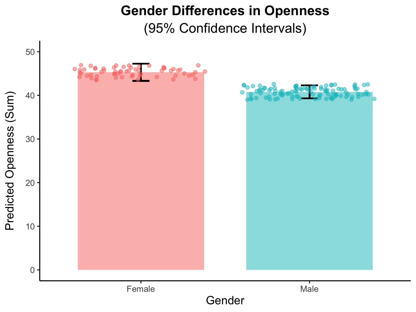
tidyr
Now, in utilizing functions from the tidyr package in Tidyverse, we can make more complex transformations to the data frame to answer more questions about our data.
For this, let’s focus on Neuroticism, the trait revolving around the tendency to experience and regulate negative emotions. Neuroticism has been found to be positively associated with Internet addiction (Kayiş et al., 2016), and people high in Neuroticism tend to use social media to find support (Tang et al., 2016).
So, we can hypothesize that Neuroticism will be positively associated with having more online, Steam friends. I ran the code, and it is!
Creating composite scores
However, while using the sum of personality items to make a trait score is a simple and intuitive metric, that is not what is typically used by personality researchers. Instead, we use composite scores to make trait scores, which is the average score across the item responses.
In addition, the 12 items that correspond to each of the 5 personality traits also belong to different facets: sub-domains within each trait. The BFI-2 measures 3 facets per personality trait (which can be seen by the lower-case letter at the end of each item name), with 4 items for each trait tapping into each related facet. For Neuroticism, Anxiety, Depression, and Emotional Volatility are the different facets.
To look at all of these different constructs, we need to create composite scores for each, and we can do this using pivot_longer().
First, let’s look at how our wide data frame looks:
print(china_sum_2[1:10, c(1, 8, 13, 18, 23)])## # A tibble: 10 × 5
## id N_1_a N_2_d N_3_e N_4_a
## <dbl> <dbl> <dbl> <dbl> <dbl>
## 1 1 1 1 1 2
## 2 2 2 2 3 4
## 3 3 3 2 3 3
## 4 4 3 2 3 3
## 5 5 4 3 2 5
## 6 6 4 3 3 2
## 7 7 2 2 2 4
## 8 8 3 2 1 4
## 9 9 4 4 3 3
## 10 10 3 2 4 4Now, let’s see what pivot_longer() does, making a data frame with only
our Neuroticism items using select().
#remember to also include our grouping variable "id"
neuro_long <- china_sum_2 |>
  select(id, starts_with("N_")) |>
  pivot_longer(
    cols = -id,
    names_to = "item",
    values_to = "score"
  )

print(neuro_long[1:20, ])
## # A tibble: 20 × 3
## id item score
## <dbl> <chr> <dbl>
## 1 1 N_1_a 1
## 2 1 N_2_d 1
## 3 1 N_3_e 1
## 4 1 N_4_a 2
## 5 1 N_5_d 1
## 6 1 N_6_e 1
## 7 1 N_7_a 2
## 8 1 N_8_d 1
## 9 1 N_9_e 1
## 10 1 N_10_a 2
## 11 1 N_11_d 1
## 12 1 N_12_e 1
## 13 2 N_1_a 2
## 14 2 N_2_d 2
## 15 2 N_3_e 3
## 16 2 N_4_a 4
## 17 2 N_5_d 3
## 18 2 N_6_e 3
## 19 2 N_7_a 2
## 20 2 N_8_d 3Now we have a data frame with 2,016 observations, and the data frame looks A LOT different!
To get facet scores, R needs to know which items belong to which facet
of Neuroticism. We, therefore, need to separate the ending letter from
each item into another column using another tidyr function,
separate():
facet_long_1 <- neuro_long |>
  separate(col = item,
           into = c("item", "facet"))
## Warning: Expected 2 pieces. Additional pieces discarded in 2016 rows [1, 2, 3, 4, 5, 6,
## 7, 8, 9, 10, 11, 12, 13, 14, 15, 16, 17, 18, 19, 20, ...].print(facet_long_1[1:20, ])## # A tibble: 20 × 4
## id item facet score
## <dbl> <chr> <chr> <dbl>
## 1 1 N 1 1
## 2 1 N 2 1
## 3 1 N 3 1
## 4 1 N 4 2
## 5 1 N 5 1
## 6 1 N 6 1
## 7 1 N 7 2
## 8 1 N 8 1
## 9 1 N 9 1
## 10 1 N 10 2
## 11 1 N 11 1
## 12 1 N 12 1
## 13 2 N 1 2
## 14 2 N 2 2
## 15 2 N 3 3
## 16 2 N 4 4
## 17 2 N 5 3
## 18 2 N 6 3
## 19 2 N 7 2
## 20 2 N 8 3When we do separate() here, however, we lose some information, and R
gives us a warning telling us that this happened. Why is this
happening?
To prevent this, we will need to use separate() to split them into three
columns first, and then we can use unite() to join the trait and
item number values back together:
facet_long_2 <- neuro_long |>
  separate(col = item,
           into = c("trait", "item_number", "facet")) |>
  unite(col = "item",
        trait, item_number,
        sep = "_")

print(facet_long_2[1:20, ])
## # A tibble: 20 × 4
## id item facet score
## <dbl> <chr> <chr> <dbl>
## 1 1 N_1 a 1
## 2 1 N_2 d 1
## 3 1 N_3 e 1
## 4 1 N_4 a 2
## 5 1 N_5 d 1
## 6 1 N_6 e 1
## 7 1 N_7 a 2
## 8 1 N_8 d 1
## 9 1 N_9 e 1
## 10 1 N_10 a 2
## 11 1 N_11 d 1
## 12 1 N_12 e 1
## 13 2 N_1 a 2
## 14 2 N_2 d 2
## 15 2 N_3 e 3
## 16 2 N_4 a 4
## 17 2 N_5 d 3
## 18 2 N_6 e 3
## 19 2 N_7 a 2
## 20 2 N_8 d 3Now, we can explicitly tell R which items belong to which facet of Neuroticism, and we will use this variable to calculate facet-level composite scores.
You try!
We want each participant to have 3 composite (average) scores, one for each facet.
- What will we need to include in
group_by()to do this? - What operation within
mutate()will we use to make the composites? - Show the first 10 rows and all of the columns
Hint: Remember when we used group_by(id) to get the correct column of
personality score sums, per person.
By using group_by(id, facet), we group by both of these variables to get
a composite score of each facet that within each participant’s own data.
We are not done, however, as there is some unnecessary repetition going on in the facet_comp variable. What repetition is going on?
We can take the mean of facet_comp, grouping by id and facet, again, which will give us a single score for each facet within each participant:
facet_long_4 <- facet_long_3 |>
  group_by(id, facet) |>
  summarise(
    facet_comp = mean(facet_comp, na.rm = TRUE)
  )

print(facet_long_4[1:10, ])
## # A tibble: 10 × 3
## # Groups: id [4]
## id facet facet_comp
## <dbl> <chr> <dbl>
## 1 1 a 1.75
## 2 1 d 1
## 3 1 e 1
## 4 2 a 2.5
## 5 2 d 3
## 6 2 e 2.75
## 7 3 a 3
## 8 3 d 2
## 9 3 e 3.25
## 10 4 a 3.25Why does the mean() function work in this way?
Great! Now, we need to move the facets into columns using
pivot_wider(), which will widen the data frame from the long format
we transformed it into.
Then, we can use mutate() to get participant’s overall Neuroticism
composite score by getting the mean of the 3 facet means, per person:
Change this around
composite_final <- facet_long_4 |>
  pivot_wider(
    id_cols = id, #specifying the id column that identifies each observation
    names_from = facet,
    values_from = facet_comp
  ) |> #can use pipe here to go into the next operation
  group_by(id) |>
  mutate(
    Neuro_comp = rowMeans(across(c(a:e)), na.rm = TRUE)
  ) |>
   #we can change the names to be more informative
   rename(
     Anxiety = a,
     Depression = d,
     Volatility = e
   )

print(composite_final[1:10, ])
## # A tibble: 10 × 5
## # Groups: id [10]
## id Anxiety Depression Volatility Neuro_comp
## <dbl> <dbl> <dbl> <dbl> <dbl>
## 1 1 1.75 1 1 1.25
## 2 2 2.5 3 2.75 2.75
## 3 3 3 2 3.25 2.75
## 4 4 3.25 2.5 2.75 2.83
## 5 5 3.75 2.25 2 2.67
## 6 6 3 3.25 2.75 3
## 7 7 2.75 2 1.75 2.17
## 8 8 3.75 3 2 2.92
## 9 9 4 4.25 3.5 3.92
## 10 10 3.5 3.25 3.75 3.5You try!
How would I pivot_longer() this final
data frame, with the facet columns and trait column together? Call this long_final.
Massive shout out to the Fall 2025 AI Derek Simon for creating this excellent Practice Set!