Practice Set: Writing Custom Functions
Writing Functions

By now we’re very familiar with how to use functions from base R and installed packages. Before we start creating our own functions, let’s review what functions are composed of:
- Function name: The name of the function, which is used to call the function after it is defined (for example, ‘head’ is the name of the
head()function). - Arguments: Arguments are placeholders. If arguments are a defined part of a function, then values (typically) must be assigned to them. Arguments can also have default values, in which case values may not need to be designated.
- Function body: The body of a function is a collection of statements that determine what the function does.
- Return value: The return value of a function is the last expression in the function body to be evaluated. It is whatever is output by the function.
The syntax for defining a function is as follows:
function_name <- function(arg_1, arg_2, ..., arg_x) {
  Function body
  return(your_output)
}
FYI: Functions technically don’t have to have defined arguments. However, in most cases arguments are helpful and/or necessary to make a function generalizable.
For example, maybe we ran a study with 50 subjects, and subjects with odd number IDs were randomly assigned to Counterbalance A and subjects with even number IDs were randomly assigned to Counterbalance B. We forgot to include this information in our data.frame (called studyData), so now it needs to be added. There are 50 participants total (50 rows), and the first few rows look like this:
##   subject    score
## 1       1 72.58587
## 2       2 75.55486
## 3       3 77.16888
## 4       4 70.30860
## 5       5 75.85825
## 6       6 76.01211
Put simply: We want to create a function that determines whether numbers in a vector are even or odd. The simplest version of this function (below) requires no arguments, and will return TRUE for subjects with even numbers and FALSE for subjects with odd numbers.
# Creating the even_odd function
even_odd <- function() {
   return((studyData$subject %% 2) == 0)
}

# Using the even_odd function
even_odd()
## [1] FALSE TRUE FALSE TRUE FALSE TRUE FALSE TRUE FALSE TRUE FALSE TRUE
## [13] FALSE TRUE FALSE TRUE FALSE TRUE FALSE TRUE FALSE TRUE FALSE TRUE
## [25] FALSE TRUE FALSE TRUE FALSE TRUE FALSE TRUE FALSE TRUE FALSE TRUE
## [37] FALSE TRUE FALSE TRUE FALSE TRUE FALSE TRUE FALSE TRUE FALSE TRUE
## [49] FALSE TRUEWhat are the components of this function?
- even_odd is the name
- No arguments are defined, thus the empty parentheses
(studyData$subject %% 2) == 0is the body of the function and is nested in…returnis your return statement
Nothing runs if you only execute the first 3 lines! You need to then call your function if you want it to actually run.
This function may be useful to someone else who regularly needs to check whether their subject numbers are even or odd… but this seems unlikely. Importantly, the function assumes that the name of the data.frame will always be studyData, and that the name of the subject column will be subject. The reason for this assumption? Because studyData and subject are hard-coded into the body of the function!
Wouldn’t it be better if the user could supply their own vector of numbers to the function? We can improve this function by specifying an argument, which we will just call x for now.
# Improving the even_odd function
even_odd <- function(x) {
   return((x %% 2) == 0)
}

# Using the even_odd function for studyData
even_odd(x = studyData$subject)
## [1] FALSE TRUE FALSE TRUE FALSE TRUE FALSE TRUE FALSE TRUE FALSE TRUE
## [13] FALSE TRUE FALSE TRUE FALSE TRUE FALSE TRUE FALSE TRUE FALSE TRUE
## [25] FALSE TRUE FALSE TRUE FALSE TRUE FALSE TRUE FALSE TRUE FALSE TRUE
## [37] FALSE TRUE FALSE TRUE FALSE TRUE FALSE TRUE FALSE TRUE FALSE TRUE
## [49] FALSE TRUE# OR, using the even_odd function for another vector of numbers
my_numbers <- 103:109
even_odd(x = my_numbers)## [1] FALSE TRUE FALSE TRUE FALSE TRUE FALSEHow else can we improve upon the current function?
Perhaps we want to return the strings "counterbalanceA" and "counterbalanceB", instead of TRUE and FALSE. Now, we need to incorporate a for loop and an if/else statement into the body of our function. (If you don’t remember the syntax for if/else statements, revisit the practice set for for loops!)
# Improving the even_odd function
even_odd <- function(x) {
  new_vector <- c() # initialize the vector
   for(i in x) {
     if((i %% 2) == 0){
       new_vector <- append(new_vector, "counterbalanceA")
     } else {
       new_vector <- append(new_vector, "counterbalanceB")
     }
   }
  return(new_vector)
}

# Let's try out our improved even_odd function, and we'll store it as a NEW column called 'counterbalance' to studyData
studyData$counterbalance <- even_odd(x = studyData$subject)
head(studyData)
## subject score counterbalance
## 1 1 72.58587 counterbalanceB
## 2 2 75.55486 counterbalanceA
## 3 3 77.16888 counterbalanceB
## 4 4 70.30860 counterbalanceA
## 5 5 75.85825 counterbalanceB
## 6 6 76.01211 counterbalanceAThe new version of this function is much more generalizable. One additional improvement we could make is to add more arguments that allow the user to choose what the labels for even and odd numbers are. Additionally, we should make sure that our arguments are clearly named!
# Improving the even_odd function (one more time!)
even_odd <- function(vectorName, evenLabel, oddLabel) {
  new_vector <- c() # initialize the vector
   for(i in vectorName) {
     if((i %% 2) == 0){
       new_vector <- append(new_vector, evenLabel)
     } else {
       new_vector <- append(new_vector, oddLabel)
     }
   }
  return(new_vector)
}

# Make new group column in studyData
# For example, maybe subjects were randomly assigned to a "training" versus a "control" group
studyData$group <- even_odd(vectorName = studyData$subject,
                            evenLabel = "training",
                            oddLabel = "control")

# View data.frame
head(studyData)
## subject score counterbalance group
## 1 1 72.58587 counterbalanceB control
## 2 2 75.55486 counterbalanceA training
## 3 3 77.16888 counterbalanceB control
## 4 4 70.30860 counterbalanceA training
## 5 5 75.85825 counterbalanceB control
## 6 6 76.01211 counterbalanceA trainingQuick Quiz
Z-scores

Now that you’re re-acquainted with the mechanics of functions, it’s time to start writing your own!
You try!
- Create a function that z-scores a vector of data. (If you don’t remember the z-score formula, look back at Week 7!)
- Your function should be named
z_score - Your function should take one argument called
values
Note, you are making this from scratch – do not include the scale function!

FYI: You can use for loops when writing functions (like the even_odd function above), and you can also nest your custom functions within a for loop!
You try!
Use a for loop with your new z-scores function to z-score all of the (numeric) columns in the iris dataset!
- Iterate across columns, saving the z-scored columns to a new data.frame called
iris_zscored. - If a column does not contain numeric values (cough
Speciescough), then it should still be added toiris_zscored, but without using the z-score function.
Hint: You may want to nest an if/else statement within your for loop!
Let’s remind ourselves of what the iris dataset looks like:
head(iris)## Sepal.Length Sepal.Width Petal.Length Petal.Width Species
## 1 5.1 3.5 1.4 0.2 setosa
## 2 4.9 3.0 1.4 0.2 setosa
## 3 4.7 3.2 1.3 0.2 setosa
## 4 4.6 3.1 1.5 0.2 setosa
## 5 5.0 3.6 1.4 0.2 setosa
## 6 5.4 3.9 1.7 0.4 setosaHint: check out is.numeric(). You put the object you want to check inside of the parentheses and it will give you a TRUE or FALSE. If you want to ask if it’s TRUE or FALSE, you put the == or != (depending on what you’re doing) outside of the parenthesis.
Ex: is.numeric(studyData$group) == TRUE is asking whether the group variable from studyData is a numeric object. The answer is no, so it returns FALSE because studyData$group is a character variable.
Making a ggplot theme

Now you’re going to create a custom ggplot2 theme and save it as a function. This theme can then be called as a layer in any future plots you make, how useful! This is especially nice if you are giving a presentation writing a paper, and you want all of your figures to have the exact same theme (remember our data visualization best practices?).
Let’s start by building on the classic ggplot2 theme (theme_classic()) – this is my personal favorite! I like that the background is plain, but the default font size is too small for my poor eyes. 👓 Also, I want to have the font in my plots be “Georgia”.
To make theme_drew(), we create a function! In the body of the function I call theme_classic() and make the changes I desire (see help pages for default settings). Note: I typically wouldn’t use serif fonts for professional plots, but they’re nice to use in examples.
FYI: I wanted to use a special font that comes from the extrafont package, so in my function I added a require() statement. This will force R to load the package, or alert the user if the package is not found. We also need to require ggplot2 since the theme_classic() function comes from there.
# Changing theme_classic into theme_drew
theme_drew <- function(){
  require(ggplot2)
  require(extrafont)
  loadfonts(device = "postscript", quiet = TRUE)
  theme_classic(base_size = 14, base_family = "Georgia")
}

# Below creates 2 plots -- one using the original `theme_classic()` and
# the other using the new custom `theme_drew()`. Then we'll combine them into
# a single figure!

plot1 <- ggplot(studyData, aes(x = score)) +
  geom_histogram(color = "black", fill = "plum4") +
  theme_classic() +
  ylim(c(0,6)) +
  ylab("Count") +
  xlab("Value") +
  ggtitle("Classic theme")


plot2 <- ggplot(studyData, aes(x = score)) +
  geom_histogram(color = "black", fill = "plum4") +
  theme_drew() +
  ylim(c(0,6)) +
  ylab("Count") +
  xlab("Value") +
  ggtitle("Drew's custom theme")

ggarrange(plot1, plot2)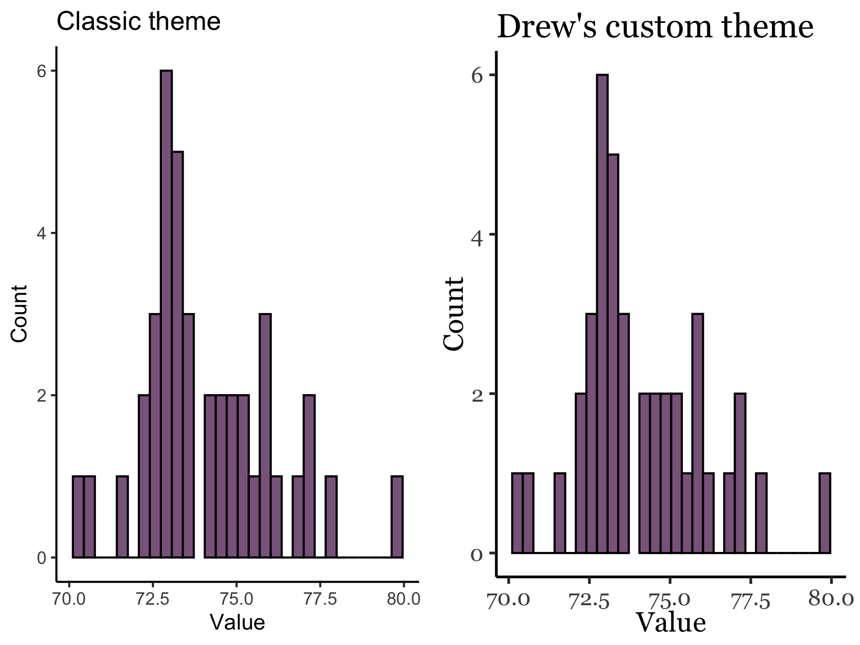
Other than the text settings, theme_drew() is just mimicking theme_classic() right now. To make larger changes, we would add the following syntax:
theme_drew <- function(){
  theme_classic(base_size = 14, base_family = "Georgia")
        theme(
            # change stuff here
        )
}
Shelly is also a big fan of the ggplot2 classic theme, but she wants the background of the plot to be transparent. On this website, it might still look white because the background is white. But when the background color is something different, she wants that to be that color. To do this, we can make changes to the classic theme, removing the inner plot background (panel.background = element_blank()) and the surrounding background (plot.background = element_blank()), both of which are usually white. Now her plot is “see through”, and the background of the plot will match the background of whatever the plot sits on top of. She also adjusts the font to be Times New Roman.
How would you know about element_blank() etc.? Professor Google! If you search for modify ggplot2 theme or something similar, a whole bunch of things should come up. If you search for R theme, you’ll have a lot more trouble.
# Changing theme_classic into theme_drew
theme_shelly <- function(){
  theme_classic()
        theme(
            panel.background  = element_rect(fill = "transparent", color = NA),
            plot.background = element_rect(fill = "transparent", color = NA),
            text = element_text(family = "Times New Roman")
        )
}

# Let's give it a go:
plot1 <- ggplot(studyData, aes(x = score)) +
  geom_histogram(color = "black", fill = "plum4") +
  theme_classic() +
  ylim(c(0,6)) +
  ylab("Count") +
  xlab("Value") +
  ggtitle("Classic theme")

plot2 <- ggplot(studyData, aes(x = score)) +
  geom_histogram(color = "black", fill = "plum4") +
  theme_shelly() +
  ylim(c(0,6)) +
  ylab("Count") +
  xlab("Value") +
  ggtitle("Shelly's custom theme")

ggarrange(plot1, plot2)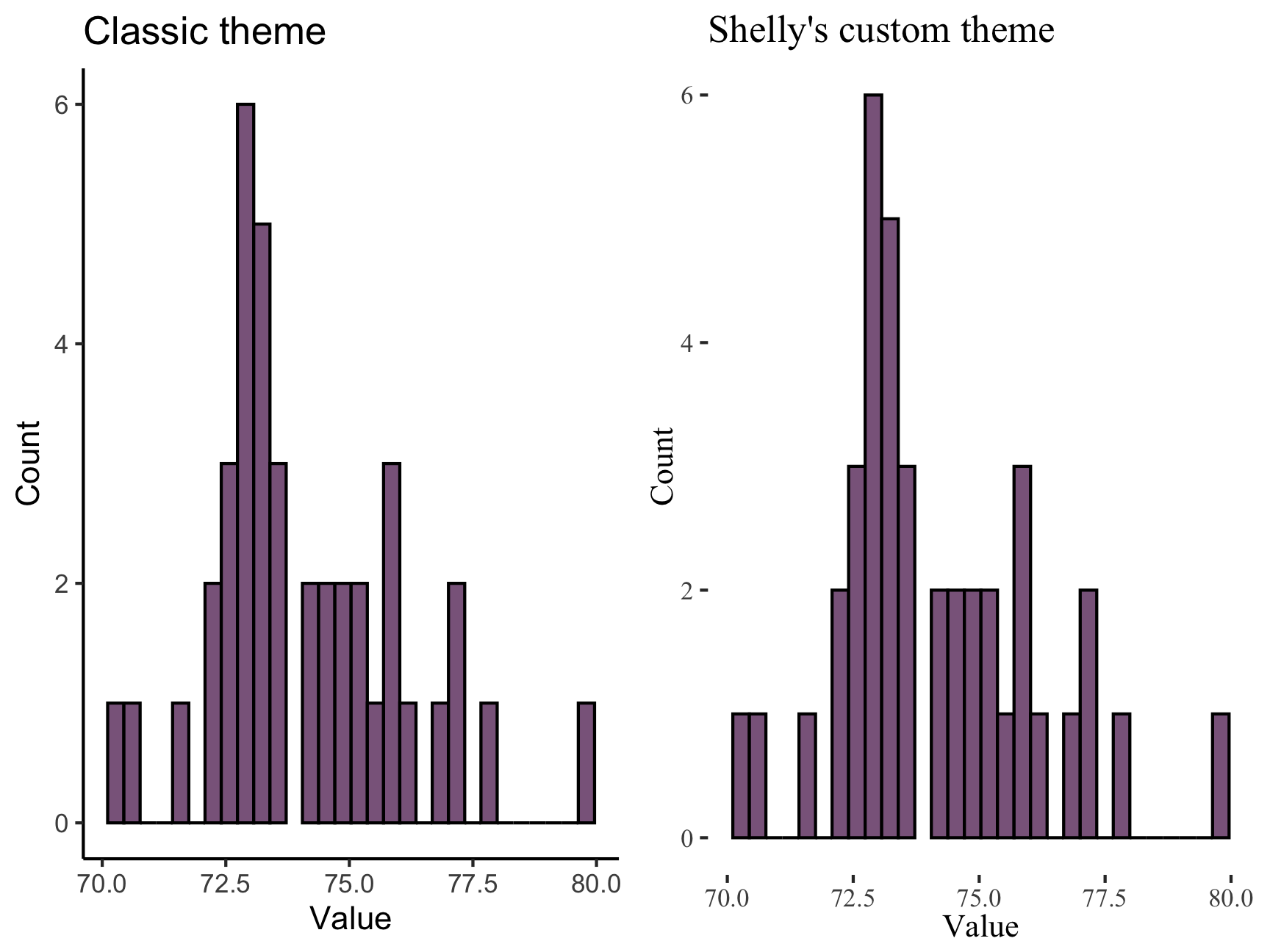
This isn’t a FYI, but just to show that the background of the plot now looks different!
![]()
You try!
Create your own theme!
- Call it
theme_new. - Then make a plot that uses this new theme to see how it looks!
There is no right or wrong answer. No solution or hints. This is a free spirited exercise
Tip: Try Googling custom ggplot2 themes! You’ll find a lot of inspiration.
Nice job finishing this practice! We hope you have fun making custom functions built for you. Once you get the hang of things and are ready to take it a step further, you can put your custom functions into your very own custom R package!
Massive shout out to the Sping 2021 AI Drew McLaughlin for creating this excellent Practice Set!