Practice Set: Regression

This time we will work with the palmer penguins dataset.

If you want to install this on your own computer, you can run the following code. It is already installed for the purposes of this website:
install.packages("palmerpenguins")Let’s take a look at our dataset!
# store it as an object so we can work with it
penguins <- palmerpenguins::penguins
kable(head(penguins))| species | island | bill_length_mm | bill_depth_mm | flipper_length_mm | body_mass_g | sex | year |
|---|---|---|---|---|---|---|---|
| Adelie | Torgersen | 39.1 | 18.7 | 181 | 3750 | male | 2007 |
| Adelie | Torgersen | 39.5 | 17.4 | 186 | 3800 | female | 2007 |
| Adelie | Torgersen | 40.3 | 18.0 | 195 | 3250 | female | 2007 |
| Adelie | Torgersen | NA | NA | NA | NA | NA | 2007 |
| Adelie | Torgersen | 36.7 | 19.3 | 193 | 3450 | female | 2007 |
| Adelie | Torgersen | 39.3 | 20.6 | 190 | 3650 | male | 2007 |
Continuous Predictor
You try!
Write a regression model and print the output for body mass in penguins predicted by bill length
Let’s interpret those coefficients!
- What does the estimate for the intercept mean?
- What does the bill length estimate mean?
- How could you calculate the \(t\)-statistic if it was not part of this output?
You try!
Now we’re going to do the following:
- Make the output prettier
- Add on extra stuff, like predicted values
- Look at fit statistics
What if our units are hard to interpret? Maybe we want to examine things in the context of standard deviation. No problem! We can standardize things!
mod2 <- lm(scale(body_mass_g) ~ scale(bill_length_mm),
           data = penguins)
summary(mod2)
##
## Call:
## lm(formula = scale(body_mass_g) ~ scale(bill_length_mm), data = penguins)
##
## Residuals:
## Min 1Q Median 3Q Max
## -2.19724 -0.55736 0.04064 0.57648 2.04109
##
## Coefficients:
## Estimate Std. Error t value Pr(>|t|)
## (Intercept) 3.793e-16 4.352e-02 0.00 1
## scale(bill_length_mm) 5.951e-01 4.358e-02 13.65 <2e-16 ***
## ---
## Signif. codes: 0 '***' 0.001 '**' 0.01 '*' 0.05 '.' 0.1 ' ' 1
##
## Residual standard error: 0.8048 on 340 degrees of freedom
## (2 observations deleted due to missingness)
## Multiple R-squared: 0.3542, Adjusted R-squared: 0.3523
## F-statistic: 186.4 on 1 and 340 DF, p-value: < 2.2e-16For a 1-SD increase in bill length, we expect weight to increase by \(b1\).
Categorical Predictor
Now what happens when we enter a categorical variable as a predictor?
You try!
Create a new model called mod3 that looks at how body mass differs by whether penguins are male and female
Let’s interpret those coefficients! - What does the intercept mean? - What does the slope mean?
Let’s get more familiar with OLS estimation and play a fun guessing game
Reporting Regression
There are many ways of reporting your models - R conveniently has some packages that make publishable tables for you. Here is an example
#install.packages("apaTables")
mod1 <- lm(body_mass_g ~ bill_length_mm, data = penguins)
apaTables::apa.reg.table(mod1)
##
##
## Regression results using body_mass_g as the criterion
##
##
## Predictor b b_95%_CI beta beta_95%_CI sr2 sr2_95%_CI
## (Intercept) 362.31 [-195.02, 919.64]
## bill_length_mm 87.42** [74.82, 100.01] 0.60 [0.51, 0.68] .35 [.28, .42]
##
##
##
## r Fit
##
## .60**
## R2 = .354**
## 95% CI[.28,.42]
##
##
## Note. A significant b-weight indicates the beta-weight and semi-partial correlation are also significant.
## b represents unstandardized regression weights. beta indicates the standardized regression weights.
## sr2 represents the semi-partial correlation squared. r represents the zero-order correlation.
## Square brackets are used to enclose the lower and upper limits of a confidence interval.
## * indicates p < .05. ** indicates p < .01.
## sjPlot::tab_model(mod1)| body_mass_g | |||
|---|---|---|---|
| Predictors | Estimates | CI | p |
| (Intercept) | 362.31 | -195.02 – 919.64 | 0.202 |
| bill length mm | 87.42 | 74.82 – 100.01 | <0.001 |
| Observations | 342 | ||
| R2 / R2 adjusted | 0.354 / 0.352 | ||
Something that was missing from the lm output – Confidence Intervals. Journals often want them reported so here is a quick way of getting them (if not using a table package that gets them for you automatically)
confint(mod1)## 2.5 % 97.5 %
## (Intercept) -195.02364 919.6371
## bill_length_mm 74.82279 100.0078When plotting using ggplot2 you’ll also get a confidence band
ggplot(penguins, aes(y = body_mass_g, x = bill_length_mm)) +
  geom_point() +
  geom_smooth(method = "lm") +
  labs(title = "Confidence Band",
       x = "Bill Length (mm)",
       y = "Body Mass (g)")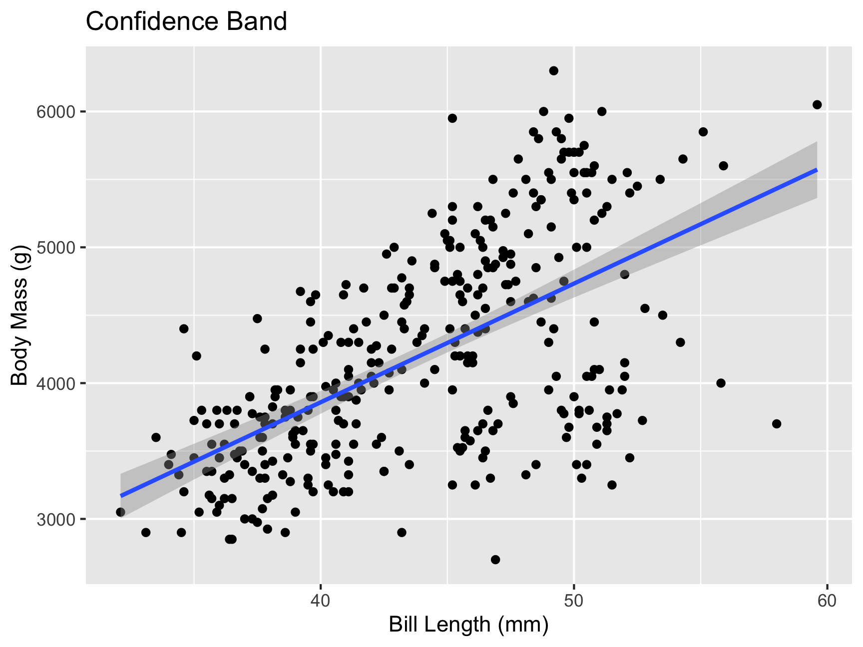
What do you notice in this plot?
Lastly, confidence bands are a little different from prediction bands. A confidence band is basically your confidence interval around the regression line. A prediction band:
- We are predicting and individual score, not the \(\hat{Y}\) for a particular level of \(X\)
- Because there is greater variation in predicting an individual value rather than a collection of individual values (i.e., the mean) the prediction band is greater
penguinsSmall = penguins %>%
  select(body_mass_g, bill_length_mm) %>%
  drop_na()

temp_var <- predict(mod1, interval = "prediction")
new_df <- cbind(penguinsSmall, temp_var)
ggplot(new_df, aes(y = body_mass_g,
                           x = bill_length_mm)) +
  geom_point() +
  geom_smooth(method = lm, se = TRUE) +
  geom_ribbon(aes(ymin = lwr, ymax = upr),
              fill = "blue", alpha = 0.1) +
  theme_classic() +
  labs(title = "Prediction Band vs. Confidence Band",
       x = "Bill Length (mm)",
       y = "Body Mass (g)")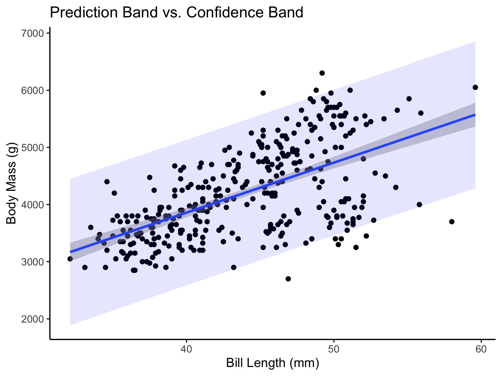
Massive shout out to the Sping 2022 AI Tabea Springstein for creating this excellent Practice Set!